Coverage Plot

A coverage plot is a genome-browser style figure: several tracks stacked vertically that all share one genomic x-axis. It is built for sequencing data, where you want to show read depth alongside variant calls and annotation lanes (amplicons, primers, genes) over the same coordinate.

CoveragePlot is a preset that assembles these tracks for you. It is not a bottom level plot type (like a scatter or a bar); it is a composite figure, in the same family as Figure. Under the hood it is built from the general TrackStack primitive (see The TrackStack primitive below), so anything the preset does you can also assemble by hand.

Type: kuva::render::coverage::CoveragePlot

Basic usage

Add one or more depth samples (each a list of (position, depth) pairs), optional typed variants, and optional feature bands. Set the locus (x range) and render. Each sample becomes a filled area depth track; variants become a tick lane with a legend; features become a labelled band lane.

#![allow(unused)]
fn main() {
use kuva::render::coverage::CoveragePlot;
use kuva::backend::svg::SvgBackend;

// (position, depth) pairs per sample
let tumour: Vec<(f64, f64)> = vec![/* ... */];
let normal: Vec<(f64, f64)> = vec![/* ... */];

let scene = CoveragePlot::new()
    .with_title("Tumour / normal coverage")
    .with_locus(1_000_000.0, 1_060_000.0)
    .with_sample("tumour", tumour)
    .with_sample("normal", normal)
    .with_variants("SNV", "#d1495b", vec![1_012_000.0, 1_028_500.0, 1_041_000.0])
    .with_variants("InDel", "#e9c46a", vec![1_033_000.0])
    .with_feature(1_005_000.0, 1_022_000.0, "amp1")
    .with_feature(1_020_000.0, 1_038_000.0, "amp2")
    .with_feature(1_036_000.0, 1_055_000.0, "amp3")
    .with_x_label("chr7 position")
    .render_sized(820.0, 380.0);

let svg = SvgBackend::new().render_scene(&scene);
std::fs::write("coverage.svg", svg).unwrap();
}

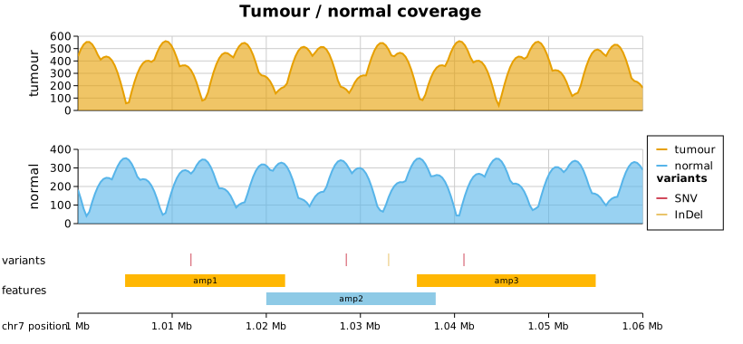
The x-axis label sits in the left gutter with the track names, and the genomic axis picks a single unit (bp, kb, Mb, or Gb) for the whole range so tick labels stay consistent.

Real data (ARTIC SARS-CoV-2)

The figure below is built from the real ARTIC nCoV-2019 example dataset (two per-pool depth files, a variant call file, and the primer scheme). It shows the pieces working together on genuine data:

• two per-pool depth tracks,
• a variant lane (SNV and InDel), coloured and listed in the legend,
• the 14 real amplicons. Because the ARTIC scheme alternates two primer pools, adjacent amplicons overlap and so tile onto two pool-coloured rows (see Feature tiling),
• a gene / ORF annotation lane, with each gene in its own colour,
• per-track legend sections on the right (samples, variants, genes).

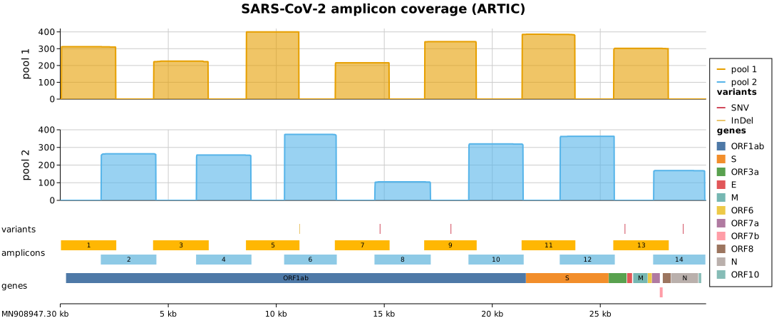
Overlapping features are handled automatically: for example ORF7a and ORF7b overlap by a few bases in the SARS-CoV-2 genome, so ORF7b is placed on its own row.

Overlaid samples

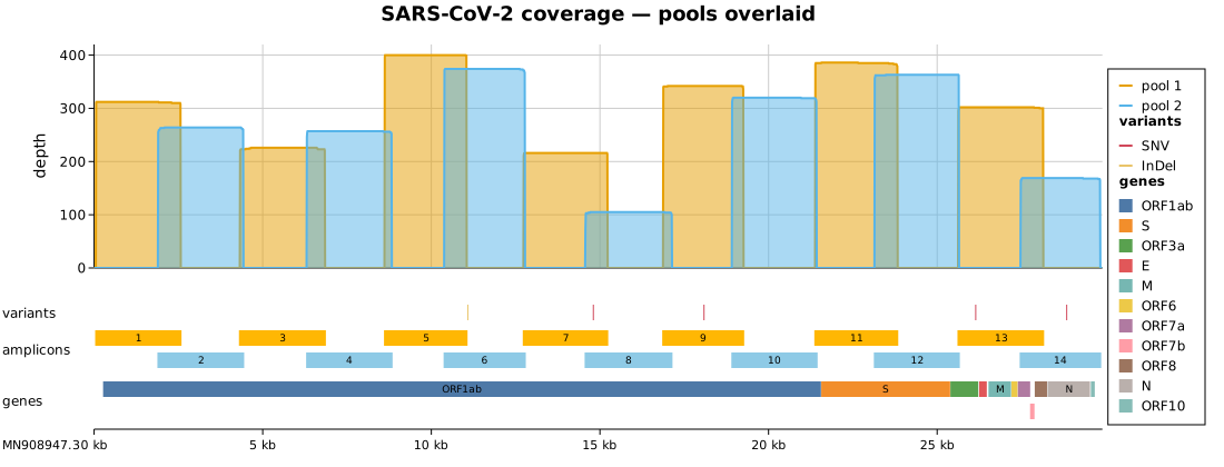
By default each sample is its own stacked track. Call .with_overlaid_samples() to draw every sample depth in one shared track on a common y-axis instead, for a direct sample-versus-sample comparison. The samples are distinguished by colour and by the legend.

#![allow(unused)]
fn main() {
use kuva::render::coverage::CoveragePlot;
let scene = CoveragePlot::new()
    .with_overlaid_samples()
    .with_sample("pool 1", vec![/* ... */])
    .with_sample("pool 2", vec![/* ... */])
    .render(1100.0);
}

Tracks and options

Feature tiling

Feature and region lanes use greedy minimum-row packing: each band takes the lowest row where it does not overlap one already placed. So N mutually overlapping bands need N rows, and no more. This gives the classic tiled-amplicon layout, where a two-pool primer scheme lands on two rows. Feature lanes colour rows by pool; region lanes colour each item individually and expose every item in the legend, so a tiny region whose label does not fit inside its band is still identifiable by colour.

Legends

Each track contributes its own titled section to a single legend on the right (samples, variants, genes, and so on), rather than merging everything into one flat list. The legend box is sized to fit the widest entry across all sections.

The TrackStack primitive

CoveragePlot is a thin preset over kuva::render::track_stack::TrackStack, a general primitive for stacking any tracks on a shared x-axis. It is not genomics specific: the same machinery drives, for example, a financial price / volume figure over a date axis. If you need a layout the preset does not offer, build a TrackStack directly:

• TrackStack::new().track(t).x_axis().render(width) assembles a stack. The x-axis is an explicit element you place with .x_axis(); tracks before it render above, tracks after render below.
• PlotTrack wraps any continuous-x Vec<Plot> (line, area, scatter, and so on) as a track.
• IntervalTrack and VariantTrack are the annotation lanes.
• AxisSpec::genomic(label) / AxisSpec::datetime(label) choose the axis formatting.
• .underlay(...) / .overlay(...) add layers that span every track (region highlights, cursors).
• .with_tick_font_family(family) sets the face for every tick label in the stack (the genomic axis and each track's y-axis), the stack-level counterpart of Layout::with_tick_font_family. A track type implements Track::set_tick_font_family to adopt it; the default ignores it, which is right for annotation lanes that draw data labels rather than ticks.

CLI

The kuva coverage subcommand builds the same figure from files. The main input is a depth table with a position column and one or more sample-depth columns; variants and features come from their own files.

kuva coverage depth.tsv --x pos --samples pool1,pool2 \
    --variants variants.tsv \
    --features amplicons.tsv --feature-name amplicons \
    --regions genes.tsv --region-name genes \
    --locus-start 1000000 --locus-end 1040000 \
    --x-label "chr7 position" --title "Amplicon coverage" \
    -o coverage.svg

Standard flags apply too (--title, --width, --height, --theme, -o, and the PNG / PDF backends via the output file extension).

The real ARTIC example files live in examples/data/covar_*.tsv:

kuva coverage examples/data/covar_depth.tsv --x pos --samples pool1,pool2 \
    --variants examples/data/covar_variants.tsv \
    --features examples/data/covar_amplicons.tsv --feature-name amplicons \
    --regions examples/data/covar_genes.tsv --region-name genes \
    --x-label "MN908947.3" --title "SARS-CoV-2 amplicon coverage" -o coverage.svg

Note: --emit-code is not supported for coverage (as with twin-y), because it is a composite figure rather than a single render_multiple call. Use the library API above to reproduce a figure in code.

See also: Manhattan Plot for GWAS results on a genomic axis, and Figure (Multi-Plot) for general multi-panel composition.