Brick Pop Plot

A brick pop plot is a population view of a single short tandem repeat (STR) locus. It shows one row per unique allele, sorted by frequency, and lines up three panels on the same rows:

• a horizontal frequency bar on the left (how common each allele is),
• a strip of metric heatboxes (per-allele values such as methylation, motif entropy, or longest pure run, each on its own colour scale),
• the motif bricks on the right (the allele's repeat structure, left anchored so expansions run off to the right).

BrickPopPlot is a composite figure, in the same family as Coverage Plot and Figure, not a bottom level plot type. It wraps a Brick Plot for the brick column and draws the frequency bar, heatboxes, colourbars, and a bottom motif legend around it. The panels stay aligned because the embedded brick's row band is pinned to the same pixel span the side panels use, so every panel agrees on the row count and row height.

Type: kuva::render::brick_pop::BrickPopPlot

Basic usage

Build a BrickPlot with your alleles (STRIGAR motif data plus names), then wrap it in BrickPopPlot, attach the per-row frequencies and metric columns, and render. Everything is positional: the frequencies and each metric's values are indexed by row, in the same order as the brick's rows. Call .sorted_by_frequency() to order every panel together so you do not have to sort each vector by hand.

#![allow(unused)]
fn main() {
use kuva::plot::{BrickPlot, ColorMap};
use kuva::render::brick_pop::{BrickPopPlot, MetricColumn};
use kuva::backend::svg::SvgBackend;
use std::collections::HashMap;

// One colour per motif, keyed by canonical k-mer, so a motif keeps its colour everywhere.
let mut colours = HashMap::new();
colours.insert("AATGG".to_string(), "#4c78a8".to_string());
colours.insert("AAGGG".to_string(), "#e45756".to_string());

let brick = BrickPlot::new()
    .with_names(vec!["allele_a", "allele_b", "allele_c"])
    .with_motif_colors(colours)
    .with_strigars(vec![
        ("AATGG:A".to_string(), "12A".to_string()),
        ("AATGG:A".to_string(), "40A".to_string()),
        ("AATGG:A,AAGGG:B".to_string(), "18A6B20A".to_string()),
    ]);

let scene = BrickPopPlot::new(brick)
    .with_title("RFC1 locus: population alleles")
    .with_frequencies(vec![0.30, 0.45, 0.25])
    .with_metric("methylation", vec![Some(0.7), Some(0.9), None], ColorMap::Viridis)
    .with_metric_column(
        MetricColumn::new("motif entropy", vec![Some(0.1), Some(0.05), Some(0.8)], ColorMap::Inferno)
            .with_range(0.0, 1.0),
    )
    .sorted_by_frequency()
    .render(880.0);

let svg = SvgBackend::new().render_scene(&scene);
std::fs::write("brick_pop.svg", svg).unwrap();
}

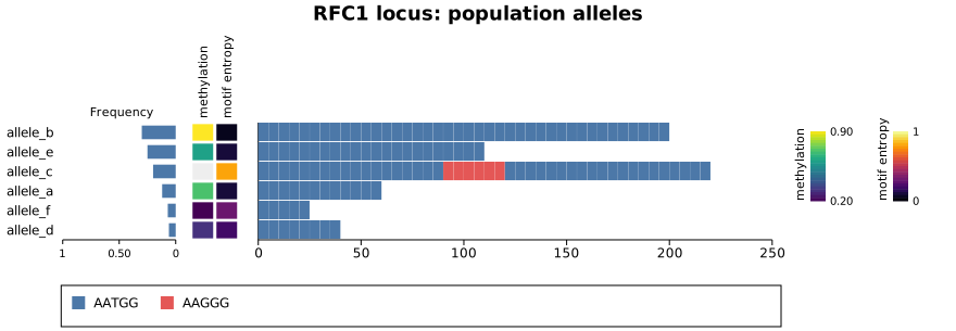
Alleles are drawn top to bottom in the order you supply, so sort by frequency first (or call .sorted_by_frequency(), which permutes the rows, the frequencies, and every metric together).

The frequency scale

The frequency bar auto-scales to [0, 1] when the values look like proportions (all in that range), and to [0, max] otherwise. This matters for small cohorts: twelve singleton haplotypes at 0.083 each render as short, equal bars rather than every bar filling to the maximum, so a polymorphic locus and a single-dominant-allele locus look obviously different and bars stay comparable across loci. Pin the scale explicitly with .with_frequency_range(vmin, vmax) when you want a fixed axis (for example counts on a shared [0, N] range).

Metrics and colourbars

Each MetricColumn is one strip of heatboxes coloured by a ColorMap. The value range is taken from the finite values unless you pin it with .with_range(vmin, vmax), and missing values (None) render in the NA colour. The colourbars are drawn side by side on the right, each with its title running vertically on its left, and the motif legend sits along the bottom (as a Legend Plot grid) so it can wrap to as many rows as a complex locus needs.

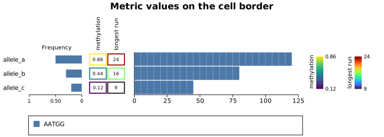
Values in the box

For a small number of alleles with tall rows, .with_metric_values(true) writes the number inside each cell and moves the heat colour to the cell border, which is easier to read exactly. Cells that are too small fall back to a solid fill automatically.

#![allow(unused)]
fn main() {
use kuva::plot::{BrickPlot, ColorMap};
use kuva::render::brick_pop::BrickPopPlot;
let brick = BrickPlot::new().with_names(vec!["a", "b"]).with_strigars(vec![("AATGG:A".to_string(), "20A".to_string()), ("AATGG:A".to_string(), "10A".to_string())]);
let scene = BrickPopPlot::new(brick)
    .with_row_height(28.0)
    .with_metric_values(true)
    .with_frequencies(vec![0.6, 0.4])
    .with_metric("methylation", vec![Some(0.86), Some(0.44)], ColorMap::Viridis)
    .render(760.0);
}

Large cohorts

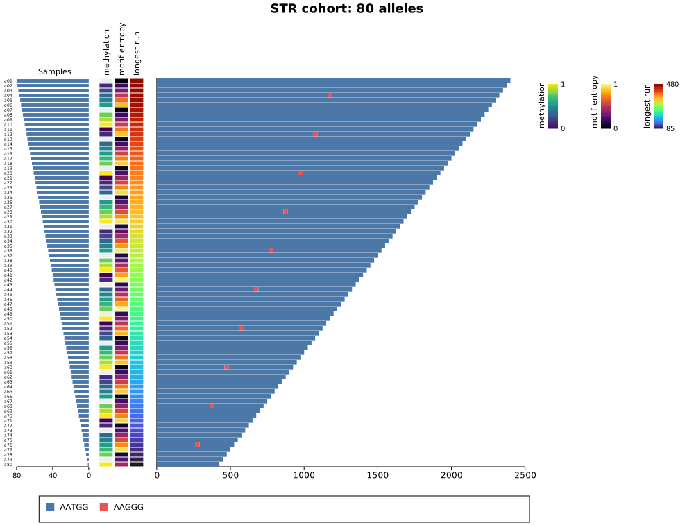
For long expansions across many alleles (RFC1, BEAN1, and similar), enable run-length merging on the brick (BrickPlot::with_merge_runs(true)) and use a small row height. Merging collapses a run of identical motifs into one bar where the per-unit width would be sub-pixel anyway, keeping very long alleles legible and cheap to draw. Allele name labels shrink to fit dense rows and are dropped when rows get too small.

Options

MetricColumn::new(label, values, colormap) builds a column; .with_range(vmin, vmax) pins its colour scale instead of auto-computing it from the data.

Note: BrickPopPlot has no CLI subcommand or --emit-code support, because it is a composite figure rather than a single render_multiple call. Use the library API above.

See also: Brick Plot for the read-level brick view and the STRIGAR format, and Coverage Plot for genome-browser style tracks on a shared locus.